Marcellus Production Outlook
April 28, 2015
Has Well Productivity Peaked in the Nation’s Largest Shale Gas Play?
The Marcellus shale gas play of Pennsylvania and West Virginia came onto the scene in 2007 in a big way and has grown to become the nation’s largest. It has accounted for much of the growth of U.S. shale gas production, and made up for declines in former shale gas giants like the Haynesville and Barnett plays of Louisiana and eastern Texas. Companies have scrambled to build pipeline infrastructure to connect the Marcellus to consumers in the U.S. northeast. Canadians, once supplied by gas from western Canada, are also looking to the Marcellus (and the much smaller Utica play in Ohio) for future supply; the pipelines that delivered gas to the east might be converted to instead deliver bitumen from the western tar sands. Companies in both the northeastern U.S. and eastern Canada are looking to build LNG terminals to export the shale gas bounty, and the first LNG export terminal on the Gulf coast will open later this year.
The prognosis for the Marcellus is therefore very important, as it is being counted on to supply abundant cheap gas to the northeast and elsewhere for decades to come. One of the big problems in figuring out what is happening with the Marcellus is the tardiness with which the states provide production data to the general public and to data vendors such as Drillinginfo, which I utilize extensively to analyze shale plays. West Virginia provides data in one-year chunks, and won’t release what happened in 2014 until mid-2015. Pennsylvania is somewhat better, releasing data in six-month chunks. In the absence of recent accurate production data, there has been much speculation on Marcellus production using proxies such as pipeline receipts and algorithms to estimate what production might be. Pennsylvania’s recent release of data from the last half of 2014, however, provides an opportunity to take an updated look at the Marcellus, considering that Pennsylvania comprises 85% of Marcellus production.
In my recent Drilling Deeper report, I looked at Marcellus data through mid-2014 with a view to determining what future production might look like. Critical observations included:
- Field decline averages 32% per year without drilling, requiring about 1000 wells per year in Pennsylvania and West Virginia to offset.
- Core counties occupy a relatively small proportion of the total play area and are the current focus of drilling.
- Average well productivity in most counties is increasing as operators apply better technology and focus drilling on sweet spots.
- Production in the “most likely” drilling rate case is likely to peak by 2018 at 25% above the levels in mid-2014 and will cumulatively produce about what the Energy Information Administration (EIA) projected through 2040. However, production levels will be higher in early years and lower in later years than the EIA projected, which is critical information for ongoing infrastructure development plans.
The following analysis provides updates using all available production data for 2014 and reveals:
- The EIA overestimates Marcellus production by between 6% and 18%, for its “Natural Gas Weekly” and “Drilling Productivity” reports, respectively.
- Five out of more than 70 counties account for two-thirds of production. Eighty-five percent of production is from Pennsylvania, 15% from West Virginia and very small amounts from Ohio and New York. (The EIA has published maps of the depth, thickness and distribution of the Marcellus shale, which are helpful in understanding the variability of the play.)
- The increase in well productivity over time reported in Drilling Deeper has now peaked in several of the top counties and is declining. This means that better technology is no longer increasing average well productivity in these counties, a result of either drilling in poorer locations and/or well interference resulting in one well cannibilizing another well’s recoverable gas. This declining well productivity is significant, yet expected, as top counties become saturated with wells, and will degrade the economics which have allowed operators to sell into Appalachian gas hubs at a significant discount to Henry hub gas prices.
- The backlog of wells awaiting completion (aka “fracklog”) was reduced from nearly a thousand wells in early 2012 to very few in mid-2013, but has increased to more than 500 in late 2014. This means there is a cushion of wells waiting on completion which can maintain or increase overall play production as they are connected, even if the rig count drops further.
- Current drilling rates are sufficient to keep Marcellus production growing on track for its projected 2018 peak (“most likely” case in Drilling Deeper).
Production
Figure 1 illustrates production from the Marcellus through December 2014 compared to estimates from the EIA. Total production was about 13.7 billion cubic feet per day (bcf/d). Estimates from the EIA for December are 14.5 and 16.1 bcf/d for its “Natural Gas Weekly” and “Drilling Productivity” reports, respectively. The Utica play of Ohio and western Pennsylvania also added an estimated 1.9 bcf/d to northeast supply in December, for a total of 15.6 bcf/d. This compares to claims of more than 19 bcf/d by some analysts, an overestimate of 22%.

Figure 1 – Production from the Marcellus based on well production data through December, 2014, for Pennsylvania, and well production data through December, 2013, for West Virginia (2014 WV production is estimated assuming the continuation of growth rates observed in the latter half of 2013). Also shown for comparison are EIA estimates from its “Natural Gas Weekly” and “Drilling Productivity” reports, and the number of producing wells.
Marcellus gas production is highly concentrated in a few counties out of the more than 70 counties that have some production, as illustrated in Figure 2. Three counties account for nearly half of the play’s production, five counties account for two-thirds, and 12 counties account for 90%. Drilling is concentrated in the top counties which have the greatest economic payback; the cheapest gas is being produced, now leaving the expensive gas for later.
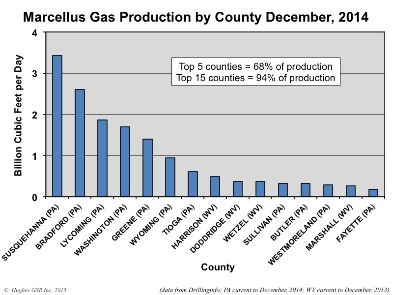
Figure 2 – Production by county for the top 15 counties in the Marcellus play illustrating the highly concentrated nature of production in sweet spots. The total number of counties with at least some Marcellus production is more than 70.
New maps published by the EIA (reproduced in Figure 3) illustrate two key Marcellus play parameters: elevation (from which one can determine depth) and thickness (an indicator of potential reservoir volume and gas concentration per unit area). These maps show the variability over the play’s extent and why it is not surprising that production is concentrated in relatively small core areas. Other parameters which factor into productivity include organic matter content, thermal maturity, presence of natural fractures, sediment composition in terms of its ability to propagate fractures, pressure, gas saturation, permeability and porosity.
Sweet spots have the most favorable combination of these parameters and are clearly concentrated in northeast Pennsylvania, northern West Virginia southwest Pennsylvania, as illustrated in Figure 4. The play’s future production trajectory depends on drilling rates and trends in well productivity as sweet spots become saturated with wells and drilling moves into lower-quality rock.
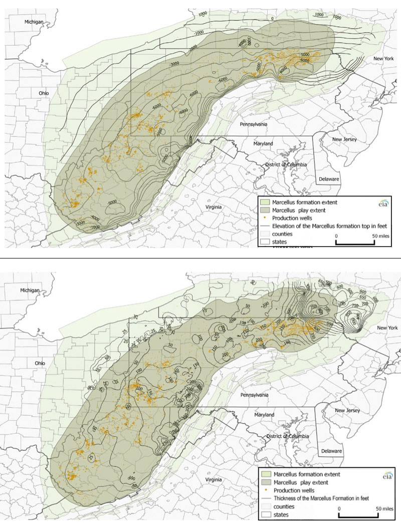
Figure 3 – Elevation (top) and thickness (bottom) of the Marcellus shale. The thickness controls the volume of the potential reservoir and potential gas distribution and the elevation determines reservoir depth which controls pressure and other critical parameters. From EIA, April, 2015.

Figure 4 – Distribution of wells in Marcellus play as of mid-2014, illustrating highest one-month gas production (from Drilling Deeper Figure 3-80).
Drilling Rates
Drilling rates and well productivity are key factors in offsetting the unceasing decline of existing wells (field decline), which in the Marcellus amounts to 32% of the play’s production that needs to replaced each year through more drilling. At the time of publication of Drilling Deeper, offsetting field decline in the Marcellus as a whole required 1,003 new wells per year, and in Pennsylvania 899 wells per year. Production is now about 10% higher but the productivity of wells has also increased on average such that the number of wells needed to offset field decline in Pennsylvania is still just over 900 per year.
Figure 5 illustrates the drilling rate in Pennsylvania and the average amount of gas added to the play’s production for each new well drilled. The current rate of about 1,050 wells per year is sufficient, should it continue, to see production rise overall until it is 15% above current levels.
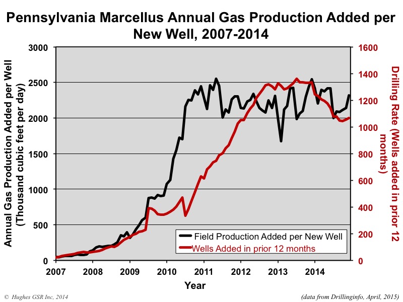
Figure 5 – Annual number of producing wells added and Marcellus play production added per new well from 2007 through December 2014 in Pennsylvania.
Another important factor is wells that have been drilled but not completed, or wells waiting on a pipeline connection. A major issue in the Marcellus has been the lack of takeaway capacity as gathering pipelines must be constructed to new wells and larger pipelines constructed to markets. Another strategy, purportedly widely used, is to drill wells without completing them, putting them in abeyance until prices are higher; as the cost of hydraulic fracturing is half or more of the total cost of a well, this practice allows producers to get a head start while rig costs are low due to the number of rigs looking for work as a result of the drop in oil prices.
Figure 6 illustrates a comparison of the rate at which wells are spudded (based on well permits) and the rate at which new producing wells are added to the play. From this it is apparent that a large backlog of drilled but not connected wells was worked off in late 2012 through 2013; the backlog has since grown again, however, with 550 more wells drilled than connected in the 12 months prior to December, 2014. The current rig count in the Marcellus is down 50% from its highs in early 2012, so even with improved rig efficiency and the ability to drill more wells per unit of time, falling rig count will ultimately limit drilling rates and impact play production.

Figure 6 – Comparison of the annual rate of wells spudded to producing wells added each year to the Marcellus in Pennsylvania, illustrating the backlog of wells waiting to be connected to production infrastructure.
Well Productivity
Well productivity is key to maintaining and growing Marcellus production, which is a function of new well productivity times drilling rate minus field decline, and to the economics of drilling the wells. We were told the following at this year’s Ceraweek conference by a Marcellus operator:
Not only are we drilling longer wells, not only are we drilling them more cheaply, but we’re getting more recovery. Today, we’re drilling the best wells we’ve ever drilled. Some of it is advances in technology. Some of it is advances in our ability, and some of it is geology — we’re in areas where we have the ability to drill longer laterals. So you can see the problem. As gas prices come off… we continue to do better and better at drilling wells.
Is this really true? The answer varies depending on where an operator’s land holdings lie and the maturity of their development. Figure 7 illustrates daily well productivity over the highest month, first 6 months, first 12 months and first 24 months for all producing wells drilled in the Marcellus in Pennsylvania from January 2010 to December 2014. It is certainly true that productivity has increased markedly over this period up to early 2014 but has decreased since, suggesting the tide has turned in the inexorable battle between technology and geology.
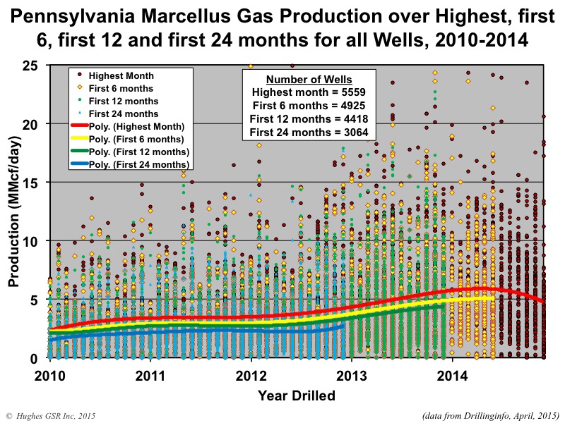
Figure 7 – Average daily production for all wells drilled in the Marcellus play between 2010 and December 2014. Dots indicate production over each well’s highest month (red), first 6 months (yellow), first 12 months (green), and first 24 months (blue). Lines indicate average daily production for all wells at these same points in time of well life (polynomial best-fit trend lines).
Figure 8 accentuates trends in well productivity in the Marcellus by fitting a moving average to the data. This figure indicates that:
- Well productivity increased by 70% between early 2012 and early 2014. This is a testament to both better technology and focusing on sweet spots.
- Productivity peaked in mid-2014 and has fallen in the last half of 2014.
- Highest month productivity is a key indicator of productivity over the longer term, as it is reflected in 6 month-, 12 month- and 24 month-average production.
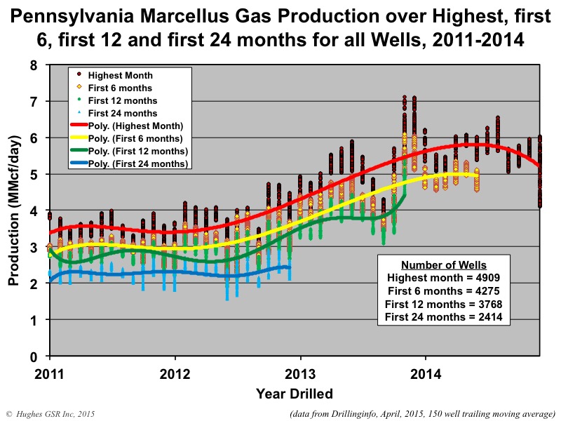
Figure 8 – Average daily production for all wells drilled in the Marcellus play between 2011 and December 2014. Data have been fitted with a trailing 150-well moving average to make the trends more apparent. Dots indicate production over each well’s highest month (red), first 6 months (yellow), first 12 months (green), and first 24 months (blue). Lines indicate average daily production for all wells at these same points in time of well life (polynomial best-fit trend lines).
It is instructive to examine comparable data for the most productive and densely drilled counties, as these will be the first to experience saturation of available drilling locations (the top four counties are analyzed below).
Susquehanna County
Susquehanna is the top producing county and also has the highest average well productivity. It is second only to Bradford County in terms of the number of wells drilled. Figure 9 illustrates average daily well production in Susquehanna County over various periods. This figure indicates that:
- Well productivity nearly doubled from early 2012 until late 2013 but has declined by nearly 20% during 2014. Susquehanna wells are still the top producers in the play.
- The fall-off in well productivity is likely due to the density of current drilling (resulting in early signs of well interference) and to drilling more marginal parts of the county.
- Geology appears to be trumping technology in Susquehanna County, which is the most productive of the play. Well density was 1.48 wells per square mile in mid-2014 (see Table 3-5 in Drilling Deeper) with the assumption that 4.3 wells per square mile could be drilled; this may be overly optimistic.
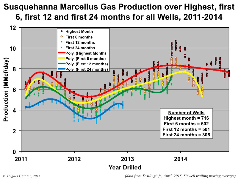
Figure 9 – Average daily production for all wells drilled in Susquehanna County between 2011 and December 2014. Data have been fitted with a trailing 50-well moving average to make the trends more apparent. Dots indicate production over each well’s highest month (red), first 6 months (yellow), first 12 months (green), and first 24 months (blue). Lines indicate average daily production for all wells at these same points in time of well life (polynomial best-fit trend lines).
Bradford County
Figure 10 illustrates average daily well production in Bradford County over various periods. This figure indicates that:
- Well productivity increased by 50% from early 2012 until early 2014 but has declined by more than 10% since then. Bradford County has the most producing wells in the play.
- The fall-off in well productivity is likely due to the density of current drilling, resulting in early signs of well interference, and to drilling more marginal parts of the county.
- Geology appears to be trumping technology in Bradford County. Well density was 1.22 wells per square mile in mid-2014 with the assumption that 4.3 wells per square mile could be drilled; this may be overly optimistic.
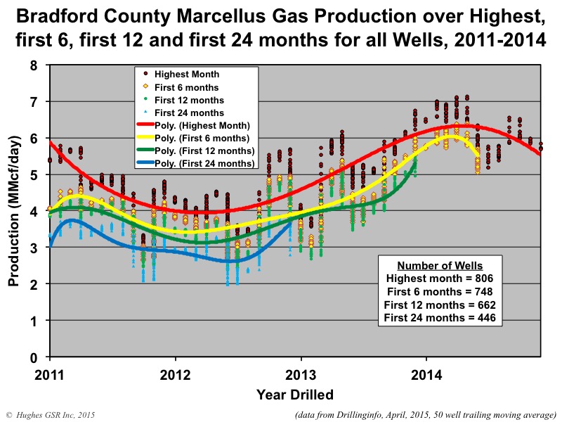
Figure 10 – Average daily production for all wells drilled in Bradford County between 2011 and December 2014. Data have been fitted with a trailing 50-well moving average to make the trends more apparent. Dots indicate production over each well’s highest month (red), first 6 months (yellow), first 12 months (green), and first 24 months (blue). Lines indicate average daily production for all wells at these same points in time of well life (polynomial best-fit trend lines).
Lycoming County
Figure 11 illustrates average daily well production in Lycoming County over various periods. This figure indicates that:
- Well productivity increased by 100% from early 2011 through 2014 but appears to be decreasing as of late 2014. Lycoming County is now second only to Susquehanna in average well productivity and third overall in production.
- It is too early to say if growth in well productivity in Lycoming County has stalled out but it appears likely. Well density was 1.35 wells per square mile in mid-2014.

Figure 11 – Average daily production for all wells drilled in Lycoming County between 2011 and December 2014. Data have been fitted with a trailing 30-well moving average to make the trends more apparent. Dots indicate production over each well’s highest month (red), first 6 months (yellow), first 12 months (green), and first 24 months (blue). Lines indicate average daily production for all wells at these same points in time of well life (polynomial best-fit trend lines).
Washington County
Figure 12 illustrates average daily well production in Washington County over various periods. This figure indicates that:
- Well productivity increased by 100% from late 2012 until early 2014 but has declined by about 10% since then. Washington County produces wet gas and most of the liquids in the Marcellus. It has generally lower well productivity than the top three counties but the liquids production has bolstered the economics.
- The fall off in well productivity is likely due to the density of current drilling, resulting in early signs of well interference, and to drilling more marginal parts of the county.
- Geology appears to be trumping technology in Washington County. Well density was 1.28 wells per square mile in mid-2014 with the assumption that 4.3 wells per square mile could be drilled; this may be overly optimistic.
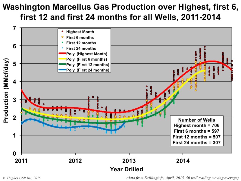
Figure 12 – Average daily production for all wells drilled in Washington County between 2011 and December 2014. Data have been fitted with a trailing 50-well moving average to make the trends more apparent. Dots indicate production over each well’s highest month (red), first 6 months (yellow), first 12 months (green), and first 24 months (blue). Lines indicate average daily production for all wells at these same points in time of well life (polynomial best-fit trend lines).
Future Production
At this point there is little reason to change the “most likely” production trajectory for the Marcellus published in Drilling Deeper (reproduced in Figure 13), other than to say it may be a bit too optimistic as drilling rates including West Virginia have fallen below the 1320 wells per year assumed (although not by much). If drilling rates fall significantly from current levels the play will peak sooner and declines will lessen after peak. Also, the observed decline in well productivity in top counties suggests that drilling densities of 4.3 wells per square mile may be too optimistic which, if so, would serve to further reduce ultimate recovery, result in more rapid declines in well productivity than assumed, and further lower production rates after peak.
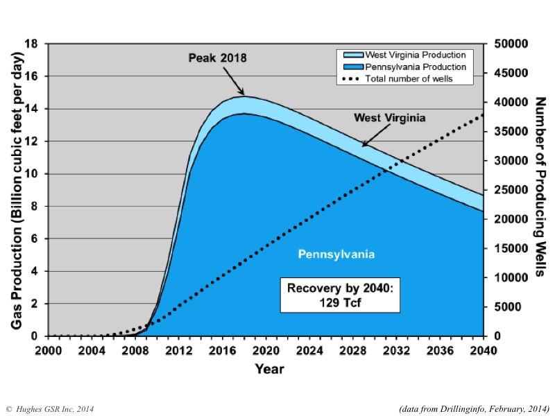
Figure 13 – Projection of future Marcellus production (“most likely” case from Drilling Deeper Figure 3-99). Cumulative recovery through 2040 is estimated at 129 tcf, which is more than 10 times the 12.6 tcf recovered to date.
Summary and Implications
Central points from this analysis include:
- The northeastern U.S. and eastern Canada are counting on abundant cheap gas from the Marcellus and Utica plays for the foreseeable future, based in part on rosy projections from the EIA that expects production to grow well into the next decade. Large investments are being made in infrastructure to transport and use this gas, including pipelines, processing plants, LNG export terminals, gas-fired generation and other residential, commercial and industrial uses. Like other shale gas plays, Marcellus wells exhibit steep production declines and the play has a field decline of 32% per year that must be offset by continuous drilling. In Pennsylvania this amounts to more than 900 wells per year simply to maintain production at current levels.
- The Marcellus play, although very large, has two-thirds of its production concentrated in 5 of 70+ counties. Although top counties have generally seen impressive increases in new well productivity over the past three years due to improved technology, most have exhibited declines in well productivity in 2014, with the top county, Susquehanna, down 20%. This is likely a result of well interference and/or moving to poorer quality locations within these counties, which suggests the assumption of a final well density of 4.3 wells per square mile may be too optimistic.
- Although production will likely grow over the next two years, barring a radical reduction in drilling rates from current levels, projections of a peak in 2018 appear on track, followed by a terminal decline (which assumes gradual increases in price; sudden major increases in price could temporarily check this decline if reflected in significantly increased drilling rates). The backlog of wells waiting on connection to infrastructure will shield production from falling for some months should there be a large drop in rig count.
- Industry invariably drills its best prospects first, hence the cheapest gas is being exploited now. Infinite faith in technology cannot make up for the realities of geology. These realities are showing up now in the most productive counties.
- As for the massive investments in infrastructure on the assumption of cheap and abundant gas for the foreseeable future – CAVEAT EMPTOR.
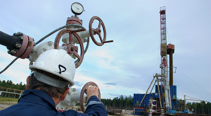
image credit: Shutterstock.com
Keep the data and analysis coming. Great job!
So glad you’re out there continuing to do this important research. A sincere thanks.